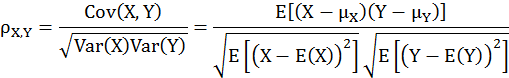
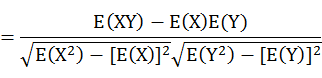
Coefficients of Correlation and Covariance

Coefficients of Correlation and Covariance

population pearson correlation coefficient

sample pearson correlation coefficient

sample covariance:

Regarding longitudinal data, the correlation matrix would be

Here j=1….t as a time point at i=1….n subject. For example a longitudinal data set:

head(obs.matrix)

  wt.2  wt.3 wt.0   wt.1 wt.4

3  13.1  13.8 NA     NA NA

6  15.8  16.2 14.9   15.1 NA

20 NA     NA NA    NA 13.3

21 14.3  14.9 14.2   14.3 NA

27 14.9  NA NA      14.7 16.0

40 NA    NA NA     NA 13.3

dim(obs.matrix)

[1] 87  5

There is correlation matrix using the function cor(method='pearon'). The correlation matrix is symmetric matrix with 1 diagonal. 
correlation coefficient ranges from -1 to 1. r=1 means perfect linear relation, and r=0 indicate no linea correlation, 
and r=-1 indicates Y would increase with X decrease.

cor.matrix<-round(cor(obs.matrix,use="pairwise.complete.obs"),3)

cor.matrix

     wt.2 wt.3  wt.0 wt.1 wt.4

wt.2 1.000 0.965 0.963 0.964 0.973

wt.3 0.965 1.000 0.971 0.943 0.966

wt.0 0.963 0.971 1.000 0.955 0.946

wt.1 0.964 0.943 0.955 1.000 0.934

wt.4 0.973 0.966 0.946 0.934 1.000

There is covariance matrix using the function cov(method='pearon').:

cov.matrix<-round(cov(obs.matrix,use="pairwise.complete.obs"),3)

cov.matrix

     wt.2 wt.3  wt.0 wt.1 wt.4

wt.2 3.008 3.054 2.849 2.824 3.120

wt.3 3.054 3.932 2.912 2.794 3.831

wt.0 2.849 2.912 2.820 2.492 2.965

wt.1 2.824 2.794 2.492 2.644 2.802

wt.4 3.120 3.831 2.965 2.802 3.720

The next, I would like to show how to calculate correlation coefficient between two time point wt.2 and wt.3.  
Here is the scatterplot.

plot(wt.2~wt.3, data=obs.matrix)

r=cor(obs.matrix$wt.2,obs.matrix$wt.3, use="pairwise.complete.obs")

r

[1] 0.9647316

text(12,15, bquote(italic(r)~'='~.(round(r,4))))

The correlation coefficient between wt.2 and wt.3 is r=0.9647316 and covariance cov=3.054.

> #remove NA

> sub<-obs.matrix[!(is.na(obs.matrix[,'wt.2'])|is.na(obs.matrix[,'wt.3'])),c('wt.2','wt.3')]

> #mean values of wt.2

> (wt.2.mean<-mean(sub$wt.2))

[1] 13.89273

> #mean values of wt.3

> (wt.3.mean<-mean(sub$wt.3))

[1] 14.51818

> #variance values of wt.2

> (wt.2.var<-var(sub$wt.2))

[1] 3.126613

> #variance values of wt.3

> (wt.3.var<-var(sub$wt.3))

[1] 3.205219

> #covariance of wt.2 and wt.3

> c=sum((sub$wt.2-wt.2.mean)*(sub$wt.3-wt.3.mean))

> c/(nrow(sub)-1) #sample covariance

[1] 3.054024

> v=sqrt(sum((sub$wt.2-wt.2.mean)^2))*sqrt(sum((sub$wt.3-wt.3.mean)^2))

> c/v #correlation coefficient

[1] 0.9647316