Logistic regression: binary regression 2x2x2 table
Consider some special cases of logistic regression model: there is two binary predictor X1 (x1=1,0)
and X2 (x2=1,0). Transform data into a 2x2x2 table:
and X2 (x2=1,0). Transform data into a 2x2x2 table:
older=0
|
older=1
| |||
bigexp=0
|
mscd=0
|
4780
|
2236
|
7349
|
mscd=1
|
101
|
232
| ||
bigexp=1
|
mscd=0
|
1802
|
1547
|
4355
|
mscd=1
|
273
|
713
| ||
6956
|
4728
|
- No interaction between two binary predictors
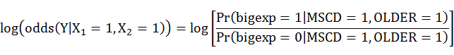
There is a formula of the model:
logit P(Y|X) = β0 +β1×MSCD + β2×OLDER
The below is coefficients estimated by glm().
> lrB=glm(data=data1,bigexp~mscd+older,family=binomial(link="logit"))
> summary(lrB)$coefficients
Estimate Std. Error z value Pr(>|z|)
(Intercept) -0.9577826 0.02700779 -35.46321 1.815505e-275
mscd 1.6549130 0.06803662 24.32386 1.096494e-130
older 0.5638298 0.04104938 13.73540 6.230701e-43
Suppose stratified 2x2 tables
Strata 1
| ||
Y=1
|
Y=0
| |
X=1
|
a1
|
b1
|
X =0
|
c1
|
d1
|
Strata 2
| ||
Y=1
|
Y=0
| |
X=1
|
a2
|
b2
|
X =0
|
c2
|
d2
|
Strata1
|
Strata2
| |||
Y=0
|
X=0
|
a1
|
b1
|
a1+b1+c1+d1
|
X =1
|
c1
|
d1
| ||
Y=1
|
X =0
|
a2
|
b2
|
a2+b2+c2+d2
|
X =1
|
c2
|
d2
| ||
a1+c1+a2+c2
|
b1+d1+b2+d2
|
Strata 1:
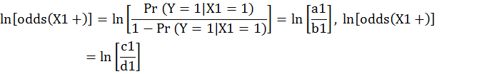

Strata 2:
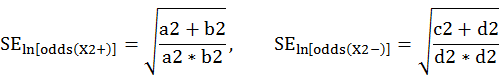

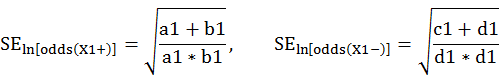
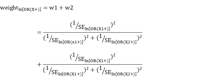
The weighted average of odds


The weighted average of odds ratio


older=0
|
older=1
| |||
bigexp=0
|
mscd=0
|
4780
|
2236
|
7349
|
mscd=1
|
101
|
232
| ||
bigexp=1
|
mscd=0
|
1802
|
1547
|
4355
|
mscd=1
|
273
|
713
| ||
6956
|
4728
|
Consider to stratify data by older
older=0
|
older=1
| ||||
bigexp=1
|
bigexp=0
|
bigexp=1
|
bigexp=0
| ||
mscd=1
|
273
|
101
|
mscd=1
|
713
|
232
|
mscd=0
|
1802
|
4780
|
mscd=0
|
1547
|
2236
|
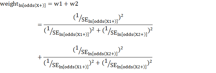
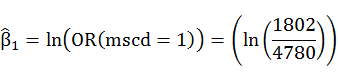
Consider β1 when mscd=1, where β1 is weighted average of odd ratio.
The values of OR are 1.645308 by hand and 1.6549130 by glm(),
and standard error are 0.06792968 by hand and 0.06803662.
The values of OR are 1.645308 by hand and 1.6549130 by glm(),
and standard error are 0.06792968 by hand and 0.06803662.


R code:
> #beta1
> OR_older0<-log((273*4780)/(1802*101))
> se_OR_older0<-sqrt(1/273+1/101+1/1802+1/4780)
> OR_older1<-log((713*2236)/(1547*232))
> se_OR_older1<-sqrt(1/713+1/232+1/1547+1/2236)
> var_cmh<-1/((1/se_OR_older0)^2+(1/se_OR_older1)^2)
> #standard error of weighted average of OR
> (SE_CMH<-sqrt(var_cmh))
[1] 0.06792968
> #weighted average of OR
> (w1<-((1/se_OR_older0)^2)/(1/var_cmh))
[1] 0.3220545
> (w2<-((1/se_OR_older1)^2)/(1/var_cmh))
[1] 0.6779455
> (OR_CMH<-w1*OR_older0+w2*OR_older1)
[1] 1.645308
Consider to stratify data by mscd. Consider β2 when mscd=1,
where β1 is weighted average of odd ratio.
The values of OR are 0.5650866 by hand and 0.5638298 by glm(),
and standard error are 0.04116406 by hand and 0.04104938.
where β1 is weighted average of odd ratio.
The values of OR are 0.5650866 by hand and 0.5638298 by glm(),
and standard error are 0.04116406 by hand and 0.04104938.
mscd=0
|
mscd=1
| ||||
bigexp=1
|
bigexp=0
|
bigexp=1
|
bigexp=0
| ||
older=1
|
1547
|
2236
|
older =1
|
713
|
232
|
older =0
|
1802
|
4780
|
older =0
|
273
|
101
|
R code
> OR_mscd0<-log((1547*4780)/(1802*2236))
> se_OR_mscd0<-sqrt(1/1547+1/4780+1/1802+1/2236)
> OR_mscd1<-log((713*101)/(273*232))
> se_OR_mscd1<-sqrt(1/713+1/232+1/273+1/101)
> var_cmh<-1/((1/se_OR_mscd0)^2+(1/se_OR_mscd1)^2)
> #standard error of weighted average of OR
> (SE_CMH<-sqrt(var_cmh))
[1] 0.04116406
> #weighted average of OR
> (w1<-((1/se_OR_mscd0)^2)/(1/var_cmh))
[1] 0.9120977
> (w2<-((1/se_OR_mscd1)^2)/(1/var_cmh))
[1] 0.08790228
> (OR_CMH<-w1*OR_mscd0+w2*OR_mscd1)
[1] 0.5650866
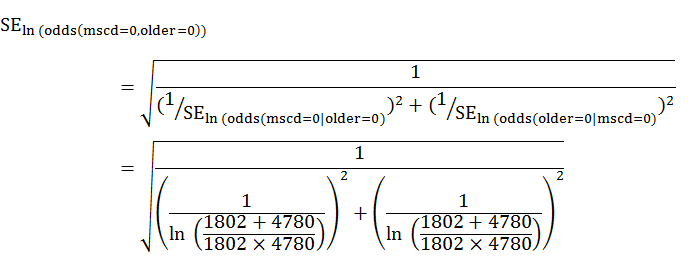
Consider the intercept that is the weighted average of log odds(bigexp|mscd=0|older=0)
and log odds(bigexp|older=0|mscd=0). The values of β0 are by -0.9755434 hand and
-0.9577826 glm(). Standard deviations are 0.02764315 by hand and 0.02700779 glm().
and log odds(bigexp|older=0|mscd=0). The values of β0 are by -0.9755434 hand and
-0.9577826 glm(). Standard deviations are 0.02764315 by hand and 0.02700779 glm().
R code
> (beta0<-log(1802/4780))
[1] -0.9755434
> (se_beta0<-sqrt((1802+4780)/(1802*4780)))
[1] 0.02764315
- interactions between two binary predictors
There is a formula of the model:
logit P(Y|X) = β0 +β1×MSCD + β2×OLDER+β3×MSCD×OLDER
There is summary by glm().
> lrC=glm(data=data1,bigexp~mscd+older+mscd*older,family=binomial(link="logit"))
> summary(lrC)$coefficients
Estimate Std. Error z value Pr(>|z|)
(Intercept) -0.9755434 0.02764313 -35.290623 8.178407e-273
mscd 1.9698947 0.11970011 16.456917 7.481555e-61
older 0.6071724 0.04310200 14.086873 4.573694e-45
mscd:older -0.4787796 0.14537749 -3.293355 9.899951e-04
The below is the mathematics deduct:

Therefore:


Then consider variance of coefficients. The value yi of the dependent variable Y follows Bernoulli trials.
The density function of binomial distribution if there is x number of success of yi given n total trials:
The density function of binomial distribution if there is x number of success of yi given n total trials:
The likelihood function
The maximum likelihood estimator of p is
The variance of odds (Delta method is used here):

Therefore


Here are the R codes:
(beta0<-log(1802/4780))
#[1] -0.9755434
(SE_beta0<-sqrt((1802+4780)/(1802*4780)))
[1] 0.02764315
(beta1<-log(273/101)-beta0)
[1] 1.969895
(SE_beta1<-sqrt((1802+4780)/(1802*4780)+(273+101)/(273*101)))
[1] 0.1197002
(beta2<-log(1547/2236)-beta0)
[1] 0.6071724
(SE_beta2<-sqrt((1802+4780)/(1802*4780)+(1547+2236)/(1547*2236)))
[1] 0.04310201
(beta3<-log(713/232)-beta0-beta1-beta2)
[1] -0.4787796
(SE_beta3<-sqrt((713+232)/(713*232)+(1802+4780)/(1802*4780)+
(273+101)/(273*101)+(1547+2236)/(1547*2236)))
(273+101)/(273*101)+(1547+2236)/(1547*2236)))
[1] 0.1453776
No comments:
Post a Comment