logistic regression: Prediction

logistic regression: Prediction

1. Predicted probability

Here is the maximum likelihood estimation :

Under the usual condition for ML:

Therefore, expected logit value follows

And 95%CI of logit value:

Suppose the function of Pr(Y|X) is always increasing or decreasing. 95%CI of expected probability:

2. 2x2 table and ROC curve

	Observation Y=1	Observation Y=0
Prediction Y=1	n11	n12	n11+n12
Prediction Y=0	n21	n22	n21+n22
	n11+n21	n12+n22

ROC stands for Receiver Operating Characteristic. ROC curve is a plot of sensitivity (true positive rate)
against 1-Specificity (false positive rate or type I error) derived from several cutting points for 
predicted value. ROC curve could be used for measuring the accuracy of the classification model 
constructed by logistic regression, CART or random forest methods. A perfect classification would be 
sensitivity=1 and (1-specificity)=0.

The area under the ROC curve (AUC) measures discrimination. The AUC is 1.0 for a perfect classifier 
and .5 for a irrelevant classifier. AUC stands for the probability that the randomly chose case (Y=1) 
has X exceeds that for a randomly chosen control (Y=0) with multiple predictors. So

3. Classification using Logistic regression

Consider a logistic regression model: logit P = Xβ. The expected value of Y is equal to Pr(Y=1|X). 
Cut-points could be used with Pr(X). If P(X) > Cp, predict subject X to be case or control. 
There are three logistic regression model of major smoking-caused disease (mscd) on 
ever-smoking(eversmk=1,0) and continuous covariate variable (lastage):

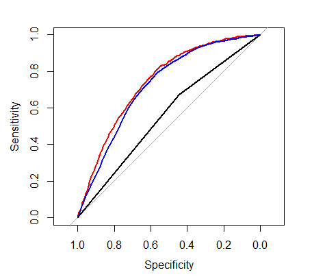
Model A: log odds (mscd=1)= β0+β1×eversmk+β2×age

Model B: log odds (mscd=1)= β0+β1×eversmk

Model C: log odds (mscd=1)= β0+β1×age

The ROC curves determined by model A-C are red, black and blue lines. 
The AUC of the model A is the highest among the three models, which indicate the best classifer.

R code:

> lr0<-glm(mscd~eversmk+ns(lastage,3), data=data1, family=binomial(link='logit'))

> lr1<-glm(mscd~eversmk, data=data1, family=binomial(link='logit'))

> lr2<-glm(mscd~lastage, data=data1, family=binomial(link='logit'))

> #ROC curves

> library(pROC)

> roc0<-roc(data1$mscd, predict(lr0, type='response'), auc=T)

> roc1<-roc(data1$mscd, predict(lr1, type='response'), auc=T)

> roc2<-roc(data1$mscd, predict(lr2, type='response'), auc=T)

> plot(roc0, col='red')

> plot(roc2, add=T, col='blue')

> plot(roc1, add=T)

The next, implement cross-validation to test the accuracy of the estimated AUC.