Tiezheng Yuan Ph.D.: Multiple Linear regression: Coefficient estimation of MLR using OLS methods

Multiple Linear regression:
Coefficient estimation of MLR

Suppose that there is linear relationship between variables X and Y. So consider a multiple variate
linear regression model (MvLR)

Remember the below formula

E(Y|X)=βX

Var(Y|X)= σ2I

Maximum likelihood function and Least square

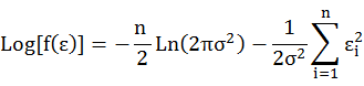
Under Gaussian multiple density distribution, εi is random independent variables. We have a Gaussian
distribution

. So

Minimize the sum of squared residuals (RSS) using Ordinary Least Square method (OLS), and
estimate unknown or observed parameters β and ε, which was denoted as

and

Due to

,
So

So,

Due to matrix calculus theorem, and X'X is symmetric matrix, so X'X=(X'X)'=XX', and (X'X)-1X'X=I.

The derivatives

set

. So

Here is a case study of multiple variables linear regression

> lm2<-lm(wt~age+ht, data=d)

> summary(lm2)

Call:

lm(formula = wt ~ age + ht, data = d)

Residuals:

Min 1Q Median 3Q Max

-2.48498 -0.53548 0.01508 0.51986 2.77917

Coefficients:

Estimate Std. Error t value Pr(>|t|)

(Intercept) -8.297442 0.865929 -9.582 <2e-16 ***

age 0.005368 0.010169 0.528 0.598

ht 0.228086 0.014205 16.057 <2e-16 ***

---

Signif. codes: 0 ‘***’ 0.001 ‘**’ 0.01 ‘*’ 0.05 ‘.’ 0.1 ‘ ’ 1

Residual standard error: 0.9035 on 182 degrees of freedom

Multiple R-squared: 0.9163, Adjusted R-squared: 0.9154

F-statistic: 995.8 on 2 and 182 DF, p-value: < 2.2e-16

> coef(lm2)

(Intercept) age ht

-8.297442239 0.005368228 0.228085501

So the coefficients of

Calculate

Based on the formula

Here are the R code for calculating

> X<-cbind(rep(1, nrow(d)), as.matrix(d[,c('age','ht')]))

> Y<-as.matrix(d$wt)

> library(MASS)

> ginv(t(X)%*%X)%*%t(X)%*%Y

[,1]

[1,] -8.297442239

[2,] 0.005368228

[3,] 0.228085501

Gauss-Markov Theorem.

Here, we am going to discuss the expected value, variance and variance-covariance of coefficients.
Gauss-Markov Theorem: OLS estimator is the Best Linear, Unbiased, and efficient Estimator (BLUE).
There are three main proofs regarding the statements.

is unbiased estimator of β:

proof

Assumption: Y=Xβ+ε, E(ε|X)=0, and X has rank k (no perfect collinearity).

Because (X'X)-1X'X=I and E(ε)=0, and Iβ=βI=β

proof variance of

has linear relationship with β

Proof

has minimal variance among all linear and unbiased estimators.

Proof variance-covariance matrix of the OLS estimates:

With linear algebra theorem COV(X)=E[(X-E(X))(X-E(X))'], and

. So

Because

and Y=Xβ+ε. So

Because

, So

Because σ2 is unknown, replace σ2 with

when n is huge. So

> #standard error of OLS_beta

> OLS_residuals<-Y-X%*%OLS_beta

> (OLS_var<-as.numeric(t(OLS_residuals)%*%OLS_residuals/182))

[1] 0.8162765

> OLS_var*diag(1, 3)

[,1] [,2] [,3]

[1,] 0.8162765 0.0000000 0.0000000

[2,] 0.0000000 0.8162765 0.0000000

[3,] 0.0000000 0.0000000 0.8162765

> #variance-covariance matrix

> (var_cov<-OLS_var*diag(1, 3)%*%ginv(t(X)%*%X))

[,1] [,2] [,3]

[1,] 0.749832532 0.0076531233 -0.0121572259

[2,] 0.007653123 0.0001034006 -0.0001341481

[3,] -0.012157226 -0.0001341481 0.0002017823

> #standard error of OLS beta

> (se_beta<-sqrt(diag(var_cov)))

[1] 0.86592871 0.01016861 0.01420501

Here are the 95% confidence intervals of

> (t95<-qt(0.975, df=182, lower.tail=F))

[1] 1.973084

> data.frame('beta'=OLS_beta, 'lower_bound'=OLS_beta-t95*se_beta,

+ 'upper_bound'=OLS_beta+t95*se_beta)

beta lower_bound upper_bound

1 -8.297442239 -10.00599239 -6.58889209

2 0.005368228 -0.01469529 0.02543175

3 0.228085501 0.20005782 0.25611318

Normality and Significance test of coefficients

The test is used to check the significance of individual regression coefficients in the multiple linear
regression model. Adding a significant variable to a regression model makes the model more
effective, while adding an unimportant variable may make the model worse. The hypothesis
statements to test the significance of a particular regression coefficient.

Under the CLM assumptions, we suppose