Multiple Linear regression: Residuals

Multiple Linear regression: Residuals

 
Here is a linear regression model in R

> lm2<-lm(wt~age+ht, data=d)

> summary(lm2)

Call:

lm(formula = wt ~ age + ht, data = d)

Residuals:

    Min     1Q Median       3Q Max

-2.48498 -0.53548  0.01508 0.51986 2.77917

Coefficients:

            Estimate Std. Error t value Pr(>|t|)    

(Intercept) -8.297442   0.865929 -9.582 <2e-16 ***

age          0.005368 0.010169   0.528 0.598

ht           0.228086 0.014205  16.057 <2e-16 ***

---

Signif. codes:  0 ‘***’ 0.001 ‘**’ 0.01 ‘*’ 0.05 ‘.’ 0.1 ‘ ’ 1

Residual standard error: 0.9035 on 182 degrees of freedom

Multiple R-squared:  0.9163,    Adjusted R-squared:  0.9154

F-statistic: 995.8 on 2 and 182 DF,  p-value: < 2.2e-16

The estimated coefficient using OLS

1. What is residual denoted as ε.

Consider a multiple variate linear regression model (MvLR). Suppose that there is linear relationship between X and Y.

                   

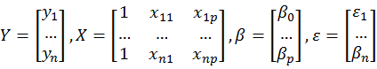
In another word, is independent random variable (iid).

There are equations if there is column matrix εnx1:

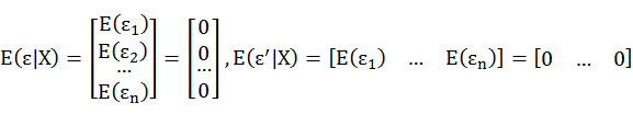
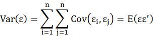
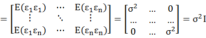
So column matrix εnx1 follows multivariates Gaussian distribution: ε ~ MVG(0, σ2I), which indicates a multivariate normal distribution of ε with mean 0nx1 and the variance-covariance matrix σ2Inxn.

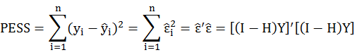
There is residuals sum of squares (RSS):

2. Estimation of residual using OLS.

Because the population residuals are unknown, so consider OLS residuals based on observed data.

Consider OLS residuals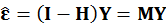

Consider another equation of

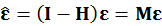
OLS residual is unbiased estimator of ε.

Proof

Proof variance of :

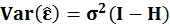
There is linear algebra theorem Var(Xv)=XVar(v)X' where v is a column and X is a matrix.

=(I-H)Var(Y)(I-H)'=Var(Y)(I-H)(I-H)'=σ2I(I-H)(I-H)= σ2(I-H)

So

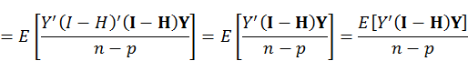
3. Estimation of variance of residuals

It is supposed that ε follow gaussian distribution, ε ~ MVG(0, σ2I), σ2 is the population variance, but it is unknown. We then estimate σ2 with . So there is a definition on , n is number of observations, and p is number of coefficients:

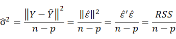
Proof is an unbiased estimator of the variance of the disturbance.

There is prediction error sum of squared (PESS) or residuals sum of squares (RSS):

So residuals standard error :

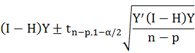
95% CI of :

The PESS estimate is useful as summary measure of a model's ability to predict new observations.

4. R Code

R code:

#matrix of independent variables

> X<-cbind(rep(1, nrow(d)), as.matrix(d[,c('age','ht')]))

> head(X)

     age ht

446 1   1 52.4

671 1   1 53.6

241 1   2 56.2

261 1   2 54.7

301 1   2 54.1

196 1   3 57.0

> dim(X)

[1] 185   3

#matrix of depencent variable:

> Y<-as.matrix(d$wt)

> dim(Y)

[1] 185   1

#degree of freedom

> (df=nrow(X)-length(coef(lm2)))

[1] 182

#OLS_beta: beta0, beta1, beta2

> (OLS_beta<-ginv(t(X)%*%X)%*%t(X)%*%Y)

            [,1]

[1,] -8.297442239

[2,]  0.005368228

[3,]  0.228085501

#hat matrix

> H<-X%*%ginv(t(X)%*%X)%*%t(X)

> dim(H)

[1] 185 185

Here is R code to calculate OLS residuals:

> residuals<-(diag(1, nrow(X))-H)%*%Y

> dim(residuals)

> #standard error of residuals

> (se_residuals<-sqrt(t(Y)%*%(diag(1, nrow(X))-H)%*%Y/df))

         [,1]

[1,] 0.9034802

> #95% CI of residuals

> (t95<-qt(0.975, df=182, lower.tail=F))

[1] 1.973084

> df<-data.frame('residuals'=residuals,

+ 'lower_bound'=as.numeric(residuals)-t95*se_residuals,

+ 'upper_bound'=as.numeric(residuals)+t95*se_residuals)

> head(df)

     residuals lower_bound upper_bound

446  0.44039334   -1.342249 2.223036

671 -0.13330852   -1.915951 1.649334

241  0.06830038   -1.714342 1.850943

261 -0.08957137   -1.872214 1.693071

301  0.04728045   -1.735362 1.829923

196  0.48046383   -1.302179 2.263106

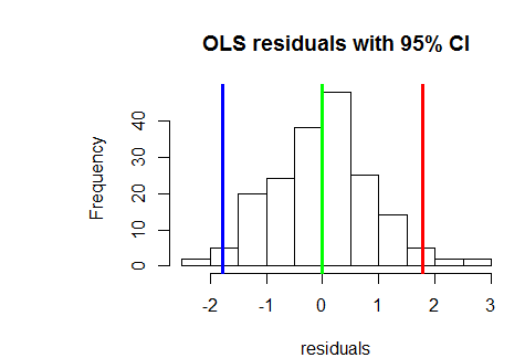
Then histogram of residuals

> hist(residuals, main='OLS residuals')

> abline(v=c(-t95*se_residuals, 0, t95*se_residuals),

+ col=c('blue', 'green', 'red'), lwd=3)